 |
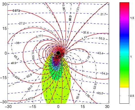
| Figure 1. Content of data tables is illustrated by this
plot, showing contour levels of various quantities. Equatorial plane of
Kerr black hole is considered (the view along rotation axis).
Observer is located towards top of the figure with inclination
of 60 deg. See the text for details. |
Previous form of data tables
This page is only good for historical reasons. It describes previous
version of the data tables which have been superseeded by their
current version (maintained largely by Michal Dovciak).
There are two global parameters: black hole angular momentum, 0<a/M<1
and observer inclination angle, 0<i<90. Non-rotating Schwarzschild
black hole has a/M=0, while extremely rotating Kerr black hole has
a/M=1; observer located along the rotation axis (pole-on) has inclination
i=0, while equatorial (edge-on) observer has i=90 deg (we
do not consider strictly edge-on position because it appears unnecessary;
in real systems radiation would be obscured by an outer torus). Below, in
Tables 1-2, each of
the figures corresponds to a certain combination of a/M and
i (Tab. 1 covers the range of radius up to 100M at low resolution
while Tab. 2 covers only the inner 50M at high resolution; otherwise
the tables arrangement is identical).
Figures illustrate the content of these tables for different parameter
values. They show a view of equatorial plane along rotation axis. Schwarzschild
coordinates are used (units of M). Observer is located on top of
the figure at spatial infinity (we do not consider strictly edge-on position
of the observer because it appears unnecessary; in real systems radiation
would be obscured by an outer torus; maximum inclination of 80 deg appears
to be suffucient). Black hole is indicated by a black circle in the centre.
An inner yellow circle is photon circular orbit, while an outer yellow circle
is the innermost stable orbit (co-rotating). All these radii are identical in
the case of extremele rotating hole. Notice that gravitational radius depends on
black-hole rotation parameter as Rg=M+(M2-a2)1/2.
Other critical orbits also depend on a. We use c=G=1
units.
Figures and tables
Each figure contains four sets of contour lines (corresponding to four
data tables):
-
Levels of redshift function are plotted with solid red curves. Values
greater than unity indicate shift of energy and observed flux towards higher
values. Doppler effect and gravitational redshift play a role here (the
latter one prevails near horizon). The curves would be symmetrical with
respect to vertical axis (butterfly-shaped) if relativistic effects were
ignored.
-
Levels of constant time delay are plotted with dashed blue lines.
They would be perfectly horizontal if relativistic effects were ignored.
Values are in geometric units and scaled with black-hole mass.
-
Levels of constant emission angle (with respect to normal to the
disc plane in a frame corotating with the disc material) are plotted with
black dash-dotted curves. Abberation and lensing play a role to determine
the values of emission angle. Far from the hole they attain the value equal
to observer inclination. Local emission angle should be considered if the
emissivity is anisotropic.
-
Levels of constant magnification (lensing effect) are plotted with
solid curves of magenta color. They have been computed by integrating geodesic
deviation equation which determines the change of cross-sectional area
between neighbouring light rays (the rays are parallel to each other at
infinity, therefore the change of area is zero in case of flat space).
Even with black-hole geometry, a significant effect occurs only for light
originating near behind the hole (i.e. the place of upper conjunction for
the observer, r<15M) and when observer is close to equatorial
plane (large inclination, i>60 deg). Far from the hole, the values
approach cosi asymptotically, which corresponds to simple effect
of geometrical projection in the euclidean geometry (without lensing);
larger values indicate light enhancement from the corresponding region
of the disc. Note: magnification is generally large only in very small
areas close to caustics; therefore contours may appear somewhat wigly if
they are drawn for very tiny magnification, especially in the case of a
small inclination; this should not introduce any significant error in spectra
computations.
Local emissivity given, the four data sets (one set for each combination
of global parameters) are sufficient to compute observed spectrum of a
source orbiting in the disc plane.
Data tables are implemented in XSPEC in such a way that the iteration
process can use all of them as necessary. Additional tables can be included,
and they can be computed with an increaed resolution, or in a different
range of radii. Hence it seems to be a good idea if the routine is prepared
for such additions/modifications, although it may be unnecessary to do
it in near future.
This (outdated) version of data tables covers equatorial plane up to r=100M
(in figures, only a smaller region is shown for clarity).
Implicit assumptions
Here we have assumed a Keplerian disc which is geometrically thin and planar
(aligned with equatorial plane), optically thick, and non-selfgravitating.
These are standard assumptions but they can be relaxed in future. We did
consider more general cases in other papers, e.g. the case of self-gravity.
Other authors discussed non-equatorial (twisted) disks or the role of highre
order images which are neglected here. For the moment we postpone additional
complications which would introduce other free parameters.
Technical notes about data tables
A Fortran code has been used to integrate geodesics (in this case, typically
105 rays for each case) and to create data tables in files.
Figures have been then produced with a Matlab script directly from these
tables, and collected in Tables 1-2 (archives contain PostScript files
and gzipped/tarred data files).
Correct values are given in the relevant range of radii; outside that
range, tables are supplemented to the rectangular
m x m matrix with the values that are evidently off.
Link to this project main page and to my homepage.