 |
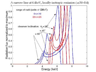
| Figure 1. An example of line profiles originating from a disc in equatorial plane of a Kerr black hole (a/M=0.4). Observer has different inclinations, as indicated in the plot. |
In other words, the main code, ky_main.f, provides a loop over polar coordinates in the disc plane (some other parameters are also specified: resolution of the grid, ranges in radii and azimuth, etc.) Data tables are needed to run this code. Given a/M and θ0, a subroutine is called that interpolates between data tables and determines redshift, light focusing, local emission angle in the disc, and time delay for each ray. Several temporary files are created that can be checked with the help of IDL and Matlab scripts.
Local emissivity can be a function of polar coordinates in the disc plane. It can also depend on local emission angle with respect to the disc normal direction, and it can be time dependent.
Figure 1 shows typical double-horn lines corresponding produced by a narrow range of radii in the disc. Typical resolutin is of the order of 104 points in the disc that contribute to the total flux; computational time is than of the order of 1 sec on an average PC workstation .
In order to test the code accuracy we computed a line with different resolution. Figure 2 shows the case of observer inclination 65 deg (equatorial plane has inclination of 90 deg). We used two different sets of tables (models "01" and "02" -- they are stored in corresponding subdirectories). Given the table set, we used different resolution of the Fortran routine (i.e. the grid of polar coordinates in the disc plane). Obviously, low resolution is less accurate and the resulting profile is somewhat wiggly.
Figure 3 illustrates a simple example of non-axisymmetric emissivity in the disc plane. Again a ring is considered as in Figure 1, but now only a segment of azimuthal angle is considered.
Current version can be downloaded of data tables and the Fortran code with related Matlab scripts (please let us know by email). Each complete set of metric tables and emissivities is stored in a single FITS format file (for example, a file containing metric tables for Kerr black hole plus emissivities for the lamp-post model). Present computations can be compared with previous results.
|
| Figure 1. An example of line profiles originating from a disc in equatorial plane of a Kerr black hole (a/M=0.4). Observer has different inclinations, as indicated in the plot. |
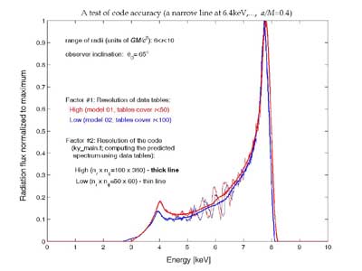 |
| Figure 2. One case has been selected from Fig. 1 and computed with different resolutions to test the code accuracy. |
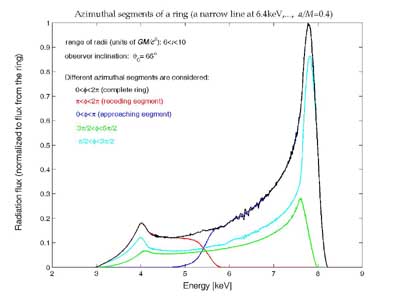 |
| Figure 3. An example of line profiles originating from an azimuthal segment of the disc. |